Best Tips About How To Build A Pareto Chart In Excel

To make a pareto chart, you need to prepare your dataset first. How to add chart elements to a pareto chart in excel step 1: Conceptdraw pro allows you to make an ms powerpoint presentation from your flowcharts in a few simple steps.

how to keep body in anabolic state how to get rid of toxic friends how to get rid of a belly how to detect sound card how to lose a big gut how to cure a hoarse voice how to draw shrubbery how to increase my blog traffic

Create A Pareto Chart In Excel (in Easy Steps)

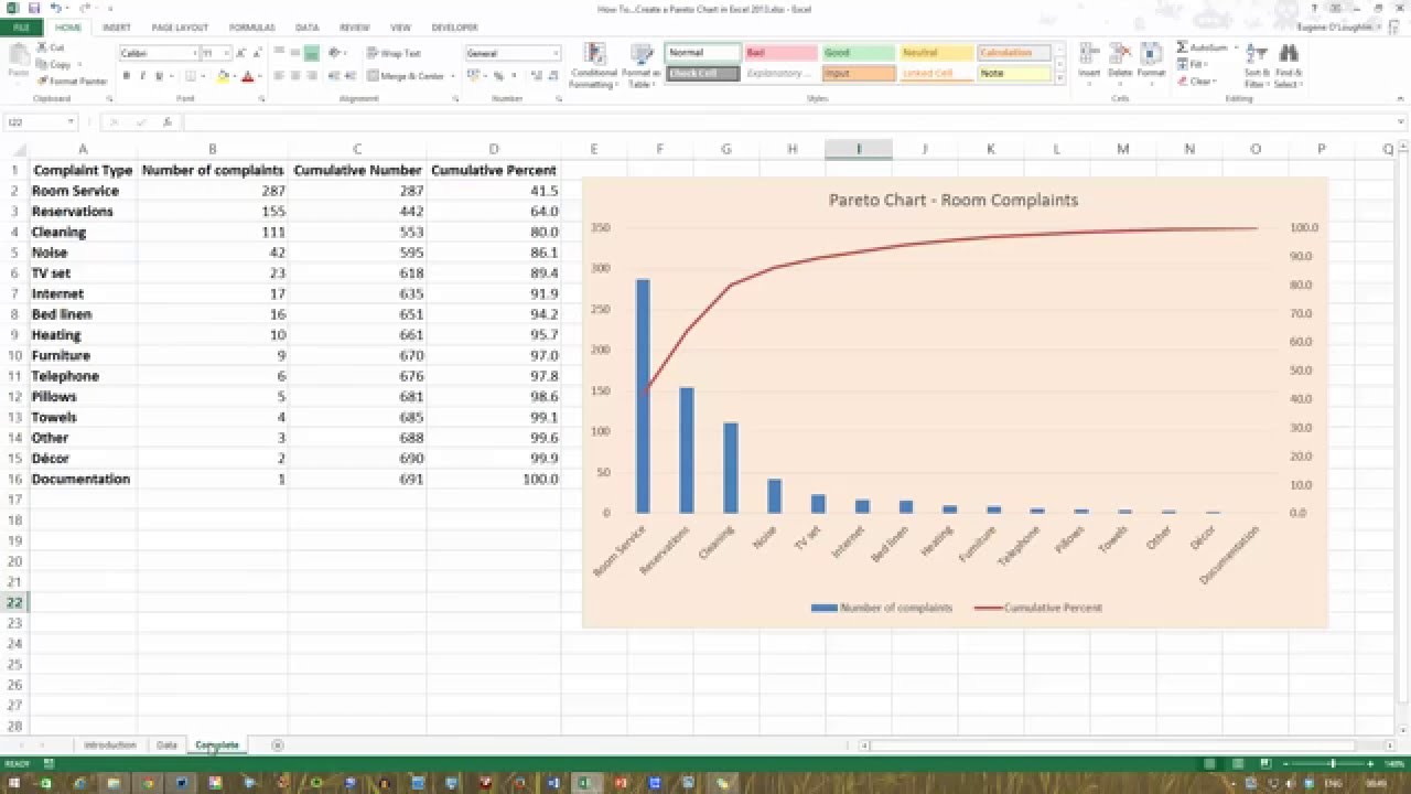
How To... Create A Pareto Chart In Excel 2013 - Youtube

How To Make A Pareto Chart In Excel (static & Interactive)

Create A Pareto Chart

How To Use The Pareto Chart And Analysis In Microsoft Excel

Later, select the base field and press ok.

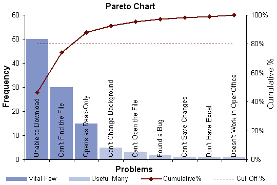
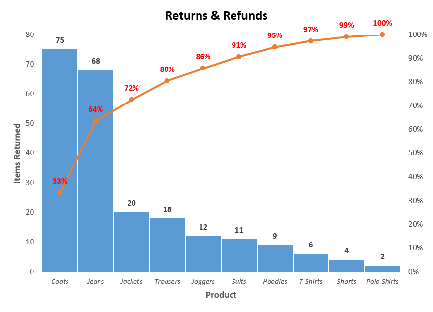
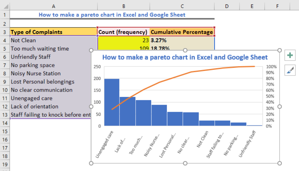
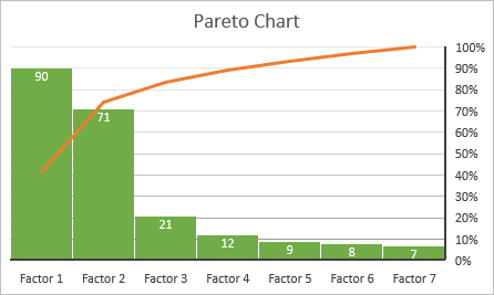
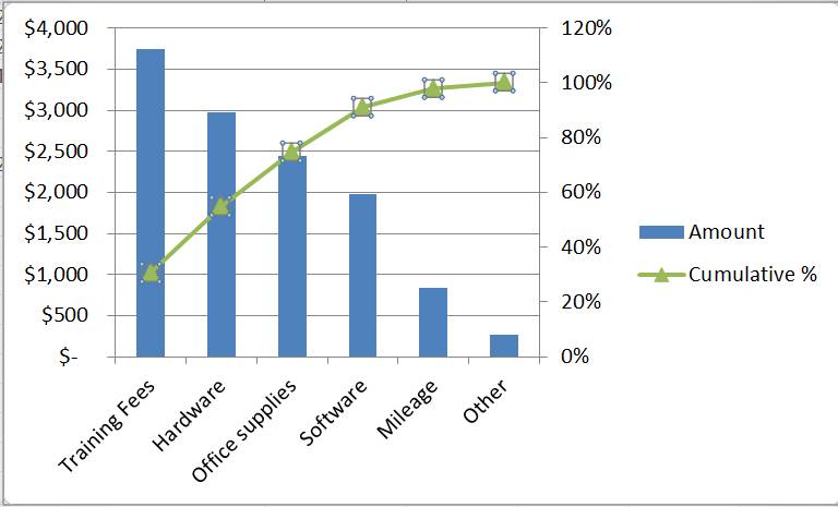
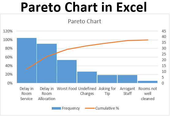
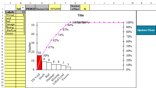
How to build a pareto chart in excel. Go to axis options in the format data series dialog box and change the value for maximum to 1.0. First, calculate the sum of all the sales amount using the. To start with cumulative amount cell.

Create a cumulative amount column. That means 64% of your. Excel will immediately insert a.

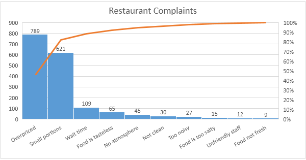
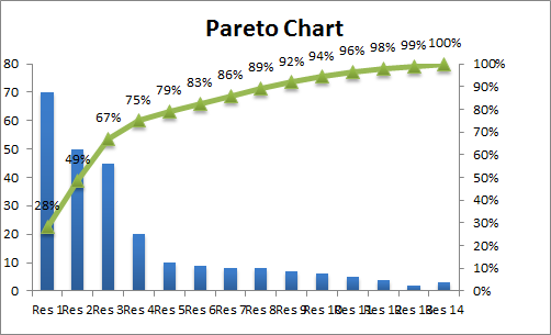
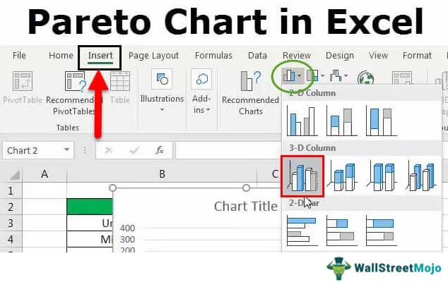
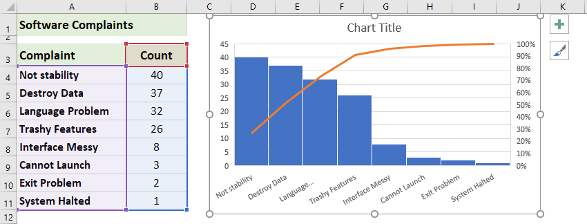
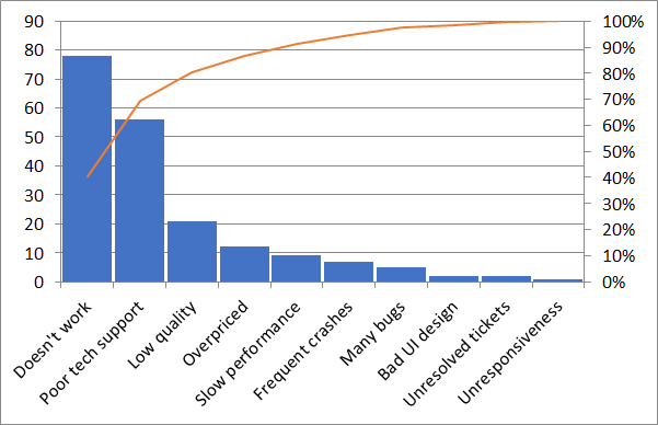
To use this option we will first select our data then will go to insert >> insert static chart >> pareto as shown in the below image. Under the histogram section, choose the pareto chart template. If you ignore the bottom 80%, 80/20 will still be true of the top 20% that’s left.

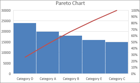
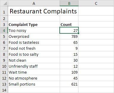
Ad smartsheet is #1 gantt spreadsheet. Remember, a pareto chart is a sorted histogram. To create a pareto chart in excel 2016 or later, execute the following steps.select the range a3:b13.on the insert tab, in the charts group, click the.

Preparing dataset to make a pareto chart. Pareto chart in excel step 2a: ️ select your range of data.

By using excel’ s inbuilt pareto chart. In this video, i am going to show you how to create a pareto chart in excel.a pareto chart is a type of chart that contains both bars and a line graph, where. Ad smartsheet is #1 gantt spreadsheet.